Teaching / Session 15 · 3 Nov 2026
Gantt Chart, Risks, Team Cost and the Full Project Estimate
Three epics and a WBS, PERT task estimates, the critical path and gates, a risk register and Monte Carlo, a team loading chart and cost, price by phase and a P80 commitment — on a robot cell with CV+AI, Jetson and ROS 2.
03.11.2026Session 15 / 15≈ 01:30 (planned)Prepared notes
Course chronology
Engineering notes
Three epics and a WBS, PERT task estimates, the critical path and gates, a risk register and Monte Carlo, a team loading chart and cost, price by phase and a P80 commitment — on a robot cell with CV+AI, Jetson and ROS 2.
Gantt and the critical path
Risks and Monte Carlo
Team, price and P80
Full session notes
Full session notes
Notes prepared before the session, continuing sessions 13–14 with a robot-cell example. There is no transcript; all numbers come from the Excel model and the Monte Carlo script and are teaching illustrations.
Session 15. From an epic plan to a full project estimate: Gantt chart, task and risk estimation, team cost
3 November 2026 · prepared session notes · ≈ 1 h 30 min (planned). These notes are not based on a transcript. They were prepared before the session at the lecturer’s request and continue the logic of sessions 01–14, above all 05, 12, 13 and 14. The running example is a robot cell with a manipulator, computer vision and AI, running on-premise on NVIDIA Jetson and ROS 2. All durations, rates and amounts are teaching illustrations, not market data. They were computed in an Excel model and a Monte Carlo script (see “Session materials”). Once the session has taken place, the actual delivery will be appended as a separate dated block; this text will not be rewritten. Editorial additions are marked separately.
0. Where this session sits in the course
Session 14 ended with a detailed 29-step plan for EPIC 1 and gates G1–G4. It also stated that an embedded project with mechanics and hardware never has a single epic — at least three. EPIC 2 and later epics, the Gantt chart, team formation and engineer profiles were announced for this session. Today we close the chain the course has been building since September:
| Question | Where it came up | What we add today |
|---|---|---|
| An estimate must be traceable: scope → WBS → roles and effort → materials → dependencies → risks → commercial estimate | Session 05 | We walk the whole chain on one example |
| E = Σ(rᵢ × tᵢ) — a simple check of a resource plan | Session 08 | From the formula to a table of roles, rates and a loading chart |
| “Feature X — 2 to 10 days at a rate of 400 dollars per day” | Session 12 | “2 to 10” is already two of the three PERT points |
| Phases, gates, cone of uncertainty, FP and T&M^ | Session 13 | How to get the phase durations (1, 3, 0.5, 7 months) from calculation rather than by assumption |
| HARA, hybrid contract, EPIC 1 plan | Session 14 | EPIC 2 and EPIC 3, Gantt chart, team, cost, full timing |
Route of the session: case → epics and WBS → task estimation → Gantt chart → risks → team and its cost → full estimate and full timing → practical tips.
1. The case: a robot cell with CV+AI, on-premise, Jetson, ROS 2
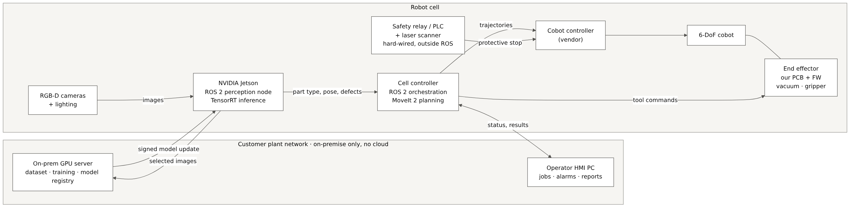
We continue the line of session 06 (a robot manipulator with a custom end effector), but take a different, more production-oriented request. The notional customer manufactures metal and plastic parts. They want a pilot cell:
- a collaborative 6-DoF robot (off the shelf, purchased) picks parts from a tray;
- cameras and a CV/AI model recognise the part type, its pose and visible defects;
- the robot sorts parts into bins, rejects separately;
- the operator sees jobs, alarms and reports on an HMI;
- all data stays in the plant: no cloud, models are trained on the customer’s own server (on-premise);
- inference runs on an NVIDIA Jetson next to the cameras;
- the integration platform is ROS 2: the customer already runs other cells on ROS 2 and wants one stack.
Constraints are not requirements
Session 06 warned that a technology name is not a requirement in itself. Here, though, Jetson, ROS 2 and on-premise come from the customer, and for good reasons: data policy, existing stack, service team. We therefore record them as design constraints with a rationale, not as functional requirements:
| ID | Type | Wording (teaching example) |
|---|---|---|
| CON-001 | Constraint | Images and models do not leave the plant network; training runs on the customer’s on-prem server |
| CON-002 | Constraint | Inference compute is an NVIDIA Jetson module in the cell cabinet |
| CON-003 | Constraint | Cell components are integrated via ROS 2 (an LTS distribution agreed with the customer) |
| SYS-PERF-001 | Requirement | Pick-and-place cycle ≤ 6 s for part types A–L under the defined test conditions |
| SYS-CV-001 | Requirement | Part-type recognition accuracy ≥ 99.0 % on the agreed test set |
| SYS-CV-002 | Requirement | Latency from frame to recognition result ≤ 150 ms (95th percentile) |
| SYS-SAF-001 | Requirement | Safety functions are defined by the cell risk assessment; they do not depend on ROS 2 or the Jetson |
Editorial note. Machinery risk assessment follows ISO 12100; safety requirements for industrial robots and robot applications are in ISO 10218-1:2025 and ISO 10218-2:2025 (third edition, February 2025). Safety functions of control systems are assessed under ISO 13849-1. The exact set of standards is decided by the safety engineer for the specific application; in the course they are only the reference basis (session 05), not a ready conclusion.
Editorial note on ROS 2. The current LTS distributions are Jazzy Jalisco (May 2024) and Lyrical Luth (22 May 2026, supported until May 2031). The Tier 1 platform for Lyrical is Ubuntu 26.04. The base Ubuntu version in the JetPack of your Jetson module may differ from the Tier 1 platform of the chosen distribution. You then have to choose between containers, a source build or another distribution. This is a classic PoC question; session 14 phrased it as “is there a proper compiler for this OS”.
2. From a list of steps to a WBS and three epics
In session 14 the EPIC 1 plan was a list of steps. To get a Gantt chart and a cost estimate, every row must become a work package with five attributes:
- ID and name — what exactly we do;
- duration — three estimates O / M / P (section 3);
- dependencies — after what the task can start;
- roles and allocation — who works on it and at what share of a full-time position (FTE);
- type — work, waiting or a control point (gate).
For our case the project splits into three epics, as session 14 forecast:
| Epic | Content | Ends with |
|---|---|---|
| EPIC 1 — “see and pick on the bench” | Discovery at the plant, system requirements, architecture, HARA, PoC (inference on Jetson; grasping with ROS 2 and MoveIt 2), MVP on one part type | Gates G1, G2, G3; a working MVP on the bench |
| EPIC 2 — “tool and cell” | Detailed requirements, component base, long-lead purchasing, end-effector board and firmware, mechanics, vendor manufacturing, assembly, cell software, dataset and model training, on-prem infrastructure | Gate G4; subsystems assembled and bench-tested |
| EPIC 3 — “integrate, validate, hand over” | Cell integration at our site, safety validation, cycle and accuracy tuning, FAT, shipping, installation, SAT and pilot run, documentation and handover | FAT, SAT, finalisation |
The full WBS has 34 work packages. Here is an abridged view (the full table with all fields is in the Excel working file):
| ID | Work package | Type | Depends on | Roles (FTE) |
|---|---|---|---|---|
| 1.1 | Discovery: site, parts, IT policy | work → G1 | — | SA 1, CV 0.5, ROS 0.5, PM 0.5 |
| 1.2 | System requirements and acceptance criteria | work → G2 | 1.1 | SA 1, QA 0.3, SAF 0.3, PM 0.3 |
| 1.3 | Architecture (ROS 2 graph, compute, network) | work | 1.2 | SA 1, ROS 0.5 … |
| 1.4 | HARA + project risk register | work | 1.3 | SAF 1, SA 0.5 … |
| 1.5 | PoC kit: Jetson dev kit, cameras, samples | waiting | 1.1 | PROC 0.2 |
| 1.6 / 1.7 | PoC-A: inference on Jetson / PoC-B: grasping with ROS 2 + MoveIt 2 | work | 1.4, 1.5 | CV 1 / ROS 1 |
| 1.8 | PoC review | work → G3 | 1.6, 1.7 | SA, PM, CV, ROS 0.5 each |
| 1.9 | MVP: one part type, bench + simulation | work | 1.8 | ROS 1, CV 1, SW 0.5, QA 0.5 |
| 2.2 | HW load estimate, component search | work → G4 | 2.1 | HW 1, PROC 0.5 |
| 2.3 | Long-lead purchasing: cobot, Jetson, safety scanner | waiting | 2.2 | PROC 0.2 |
| 2.4 → 2.7 | End-effector board → review → mechanics → review and rework | work | chain | HW, FW, ME |
| 2.8 / 2.9 / 2.10 | Board / mechanics manufacturing / standard parts purchasing | waiting | 2.7 | vendors (T&M) |
| 2.13 → 2.14 | Assembly, review, rework → FW on real hardware | work | 2.8–2.11 | TECH, FW, QA |
| 2.15 / 2.16 / 2.17 | Cell software and HMI / dataset and 3 training iterations / on-prem server | work | 1.9, 2.1 | ROS, SW, CV |
| 3.1 → 3.8 | Integration → safety → tuning → FAT → shipping → installation → SAT → handover | work / waiting | chain | all |
Role codes: PM — delivery / engineering manager, SA — system architect, ROS — robotics engineer (ROS 2, MoveIt 2), CV — CV/ML engineer, SW — software engineer (HMI, on-prem, MLOps), FW, HW, ME — firmware, hardware, mechanical engineer, SAF — safety engineer, QA — V&V engineer, TECH — assembly technician (session 14), PROC — procurement manager.
Three practical rules for building a WBS:
- Package size. A work package is estimated when it can be done and checked within a few days or a few weeks. If an engineer says “three months”, the package needs further splitting. The exception is waiting tasks: board manufacturing takes 3–5 weeks, and there is no point splitting it.
- Waiting gets its own row. Manufacturing, shipping and customs clearance have almost no effort but real calendar duration. If they are not separated out, they eat time the plan does not have.
- Integration gets its own row. The sum of subsystems is not the system: gluing them together takes real time (in our plan, package 3.1, about three weeks).
3. Task estimation: from “2–10 days” to PERT
Who estimates
Session 12 named the problem of accountability for an estimate: an external expert may underestimate a task because someone else will do it. Hence the rule: the person who will do the work estimates it, and someone who has done similar work checks it. If there is no team yet, the estimate comes from the pre-sale core team (session 06) and, where needed, paid external experts. Their estimates are marked as assumptions to be revisited after hiring.
Three points instead of one
An engineer who says “2 to 10 days” has in fact already given the optimistic (O) and pessimistic (P) estimates. What is missing is the most likely (M). PERT combines them as follows:
E = (O + 4M + P) / 6, σ = (P − O) / 6,
where E is the expected duration and σ a measure of its uncertainty. Examples from our WBS:
| Package | O | M | P | E | σ |
|---|---|---|---|---|---|
| “Feature X” from session 12 (if M = 4) | 2 | 4 | 10 | 4.7 | 1.3 |
| 1.6 PoC-A: inference on Jetson | 10 | 15 | 25 | 15.8 | 2.5 |
| 2.4 End-effector board: schematic, PCB, BoM | 10 | 15 | 22 | 15.3 | 2.0 |
| 2.8 Board manufacturing at the vendor | 15 | 20 | 30 | 20.8 | 2.5 |
| 2.16 Dataset v1 + 3 training iterations | 20 | 30 | 45 | 30.8 | 4.2 |
| 2.3 Long-lead purchasing (cobot, Jetson, scanner) | 20 | 30 | 50 | 31.7 | 5.0 |
Durations here are in working days. Note that E is always shifted from M towards P, because in engineering the risks “to the right” are longer than those “to the left”. A task cannot finish in less than zero days, but it can overrun without limit.
Editorial note. PERT (Program Evaluation and Review Technique) was developed in the late 1950s for the US Navy Polaris programme. The formula E = (O + 4M + P) / 6 approximates a beta distribution; it is not a law of nature. It is useful because it forces people to state a range and makes the asymmetry of risk visible.
Effort, duration and calendar are three different numbers
| Quantity | Unit | How to get it | Example: package 3.1 “Cell integration” |
|---|---|---|---|
| Duration | working days | PERT | E = 15.8 days |
| Effort | person-days | duration × FTE of each role (formula E = Σ rᵢ × tᵢ from session 08) | ROS 1 + CV 0.5 + FW 0.5 + HW 0.5 + TECH 0.5 + SW 0.5 = 3.5 FTE → 55 person-days |
| Calendar | date | working days from the start date, allowing for weekends, public holidays, leave | start 11.01.2027 → date from the project calendar |
If an engineer estimates in “ideal hours” — without meetings, reviews and context switches — divide the estimate by a focus factor (usually 0.7–0.8). In our model O/M/P are already given in real working days.
How to estimate AI tasks
Model accuracy cannot be estimated in days: nobody knows in advance how many days it takes to reach 99.0 % on reflective metal parts. So you estimate the experiment, not the result:
- package 2.16 is “dataset v1 + three iterations of data → training → evaluation”, time-boxed;
- the accuracy reached after three iterations goes to review: either the requirement is met, or this is risk R2 with its own plan (section 5);
- PoC-A (1.6) removes the main uncertainty earlier: whether the model fits within 150 ms on the Jetson after TensorRT optimisation.
4. The Gantt chart: dependencies, critical path, gates
How to build it
- Set the dependencies. Most are finish-to-start: task B starts after A finishes.
- Forward pass: a task’s early start ES is the latest early finish of its predecessors; early finish EF = ES + E.
- Backward pass: from the project finish backwards we get the late start LS and late finish LF.
- Float = LS − ES. Tasks with zero float form the critical path: any delay on it moves the whole project.
- Mark gates and acceptance (FAT, SAT) as milestones.
What the chart shows
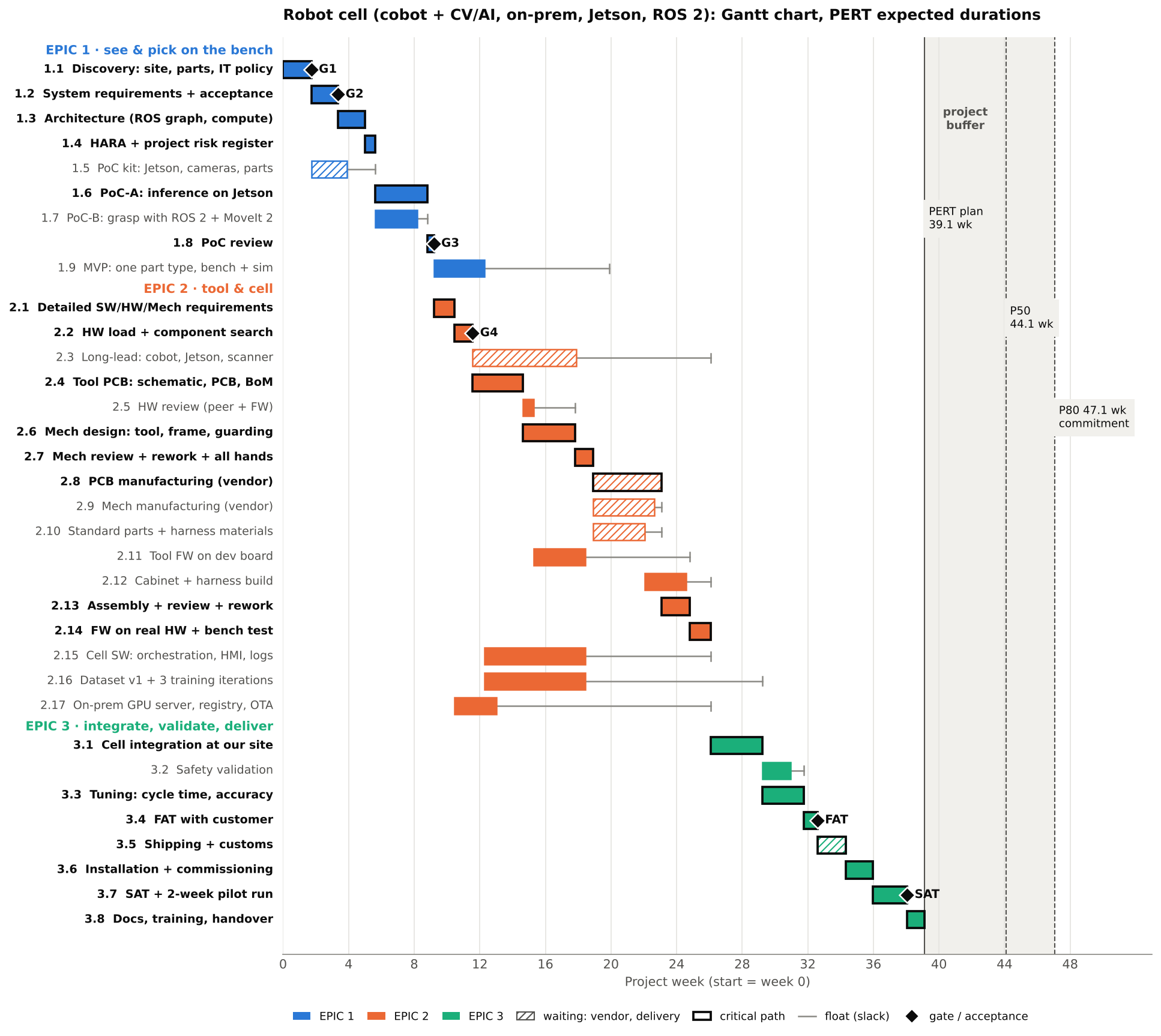
The critical path runs through hardware and mechanics, not through software:
1.1 → 1.2 → 1.3 → 1.4 → 1.6 → 1.8 → 2.1 → 2.2 → 2.4 → 2.6 → 2.7 → 2.8 → 2.13 → 2.14 → 3.1 → 3.3 → 3.4 → 3.5 → 3.6 → 3.7 → 3.8.
The critical path under PERT is 195.7 working days ≈ 39.1 weeks. Meanwhile the cell software (2.15) has 38 days of float, the dataset and training (2.16) 54 days, the on-prem server (2.17) 65 days. This illustrates the point of session 05: an embedded Gantt chart depends on things that do not speed up when you add another software engineer.
Editorial note. Brooks’s law (“adding manpower to a late software project makes it later”, F. Brooks, The Mythical Man-Month, 1975) applies here in an even stronger form: board manufacturing at the vendor will not get shorter however many programmers you add.
Long-lead items have float if you order them on time. Package 2.3 (cobot, production Jetson module, safety scanner) starts right after G4 and has 40.8 days of float. If, out of habit, the cobot is ordered after the mechanics review (2.7), this package itself becomes critical and moves the project. That is the first practical tip (section 8).
Gates on the chart:
| Milestone | After package | Working day | Week | Date (start 11.01.2027) |
|---|---|---|---|---|
| G1 — environment understood | 1.1 | 8.7 | 1.7 | 22.01.2027 |
| G2 — requirements approved | 1.2 | 16.8 | 3.4 | 03.02.2027 |
| G3 — PoC passed | 1.8 | 46.0 | 9.2 | 16.03.2027 |
| G4 — components available | 2.2 | 57.8 | 11.6 | 01.04.2027 |
| FAT — acceptance at our site | 3.4 | 163.0 | 32.6 | 26.08.2027 |
| SAT — acceptance at the plant | 3.7 | 190.3 | 38.1 | 04.10.2027 |
Everything to the right of a gate is a conditional plan. Session 13 reminded us that gates change all the rules. So we detail the near horizon (EPIC 1, to the day) and keep the far horizon in large packages. After each gate the plan is refined (rolling wave planning). This is how the cone of uncertainty narrows in practice.
5. Project risk estimation: register, reserve and Monte Carlo
HARA and the project risk register are different tables
| HARA (session 14) | Project risk register | |
|---|---|---|
| About | Hazards that the product creates for people and the system | Threats to the project’s schedule, budget and quality |
| Assessment | Severity × probability (in the course); formally S/E/C → ASIL under ISO 26262 or PL under ISO 13849 | Probability × impact in days and money |
| Output | Safety functions, requirements, PoC scope | Time and money reserve, responses, risk owners |
Both tables are built together at one meeting of the whole engineering team (package 1.4). The mechanics are the same, but they answer different questions.
Risk register for the case
| ID | Risk | Package | P | Impact, days | Impact, € | EMV, days | Response |
|---|---|---|---|---|---|---|---|
| R1 | Long-lead items slip (production Jetson, cobot) | 2.3 | 0.30 | 20 | — | 6.0 | Mitigate: order right after G4; agree a backup supplier |
| R2 | Accuracy below target on reflective parts → a fourth training iteration | 3.3 | 0.40 | 10 | — | 4.0 | Mitigate: PoC-A on the hardest parts; lighting is part of the CV subsystem |
| R3 | Second board revision (second spin) | 2.8 | 0.30 | 15 | 1,500 | 4.5 | Mitigate: two reviews (HW peer + FW) before manufacturing (session 14) |
| R4 | Customer IT security approval for the on-prem server | 2.17 | 0.40 | 10 | — | 4.0 | Accept: 65 days of float absorb it; file the request at G2 |
| R5 | ROS 2 driver for the chosen cobot immature | 1.7 | 0.25 | 8 | — | 2.0 | Avoid: choose the cobot after PoC-B; supported ROS 2 integration is a selection criterion |
| R6 | Risk assessment demands an extra safety device | 3.2 | 0.25 | 10 | 3,000 | 2.5 | Mitigate: safety engineer already in 1.2 and 1.4 |
| R7 | Key CV engineer leaves | 2.16 | 0.10 | 15 | — | 1.5 | Mitigate: pair work, documented training pipeline |
| R8 | Shipping and customs delay | 3.5 | 0.40 | 7 | 500 | 2.8 | Transfer/accept: T&M for shipping (session 14), slack in the plan |
| Total (naive EMV sum) | ≈ 1,400 | 27.3 |
EMV (expected monetary value) = probability × impact. The naive EMV sum is 27.3 days. But that is an overestimate: risks R1, R4 and R7 hit tasks with large float and do not move the project finish. So the effect of a risk on the date depends on where it sits on the Gantt chart. That is hard to compute by hand, so we simulate.
Monte Carlo: the date as a probability
The idea is simple: “play” the project 20,000 times. In each run, every duration is drawn at random from its O…P range (with a PERT distribution), every risk fires with its own probability, and the critical path is recomputed. The result is not one date but a distribution of dates.
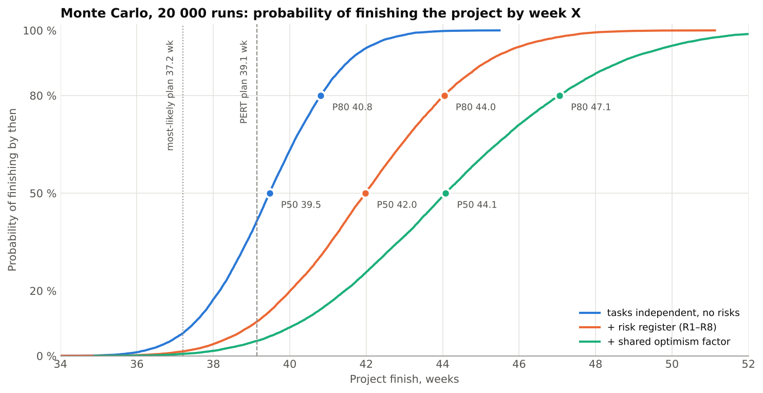
Steps from a naive date to an honest one:
| How it was computed | Working days | Weeks | Finish date |
|---|---|---|---|
| Sum of all M “one after another” (never plan like this) | 396 | 79.2 | — |
| Critical path on M (most likely estimates) | 186.0 | 37.2 | 28.09.2027 |
| Critical path on PERT E | 195.7 | 39.1 | 12.10.2027 |
| Monte Carlo, independent tasks, no risks: P50 / P80 | 197.3 / 204.1 | 39.5 / 40.8 | 13.10 / 22.10.2027 |
| + risk register R1–R8: P50 / P80 | 209.9 / 220.2 | 42.0 / 44.0 | 01.11 / 15.11.2027 |
| + shared optimism factor (0.95 … 1.0 … 1.25): P50 / P80 | 220.4 / 235.3 | 44.1 / 47.1 | 15.11 / 06.12.2027 |
Three conclusions:
- The M-based estimate is the most optimistic of the “reasonable” ones. Even without risks it has about a 7 % chance of coming true; in the full model, under 1 %. The PERT-E plan comes true in only about 5 % of runs of the full model (Fig. 15.3).
- Parallel branches push the date to the right (merge bias). The classic PERT formula for a single critical path gives σ ≈ 7.3 days and P80 ≈ 201.8 days. The simulation gives 204.1: parallel branches that become critical in some runs pull the date out. For example, PoC-B (1.7) is on the critical path in 36 % of runs, mechanics manufacturing (2.9) in 22 %.
- Independent tasks are an illusion. One team’s estimates err in the same direction: the same optimism, the same market, the same customer. A shared multiplier on all work tasks widens the distribution. That is why an experienced supplier puts a ±30 % corridor on T&M^ (session 13), even though a “clean” simulation of independent tasks gives a narrower one.
Editorial note. In PMI terms, the reserve for known risks from the register is the contingency reserve, and the reserve for unknowns is the management reserve; the latter is usually not part of the baseline and is controlled by management. The parameters of the shared optimism factor (0.95 … 1.25) in our model are a teaching assumption, not statistics. A real company calibrates it on the history of its own projects: the ratio of actual to estimated durations.
6. The team and its cost
Forming the team from the Gantt chart
Team composition is not a list of “who we would like” but a consequence of the WBS: each role appears when a work package requires it. The resource histogram is obtained by adding up the FTE of all tasks for each week.
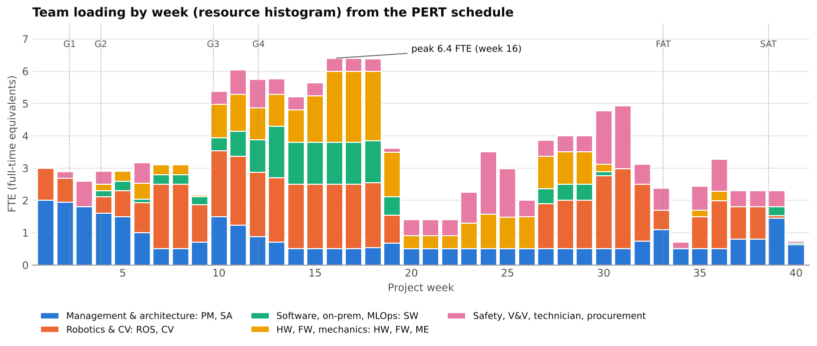
| Role | Person-days | First — last week | Peak FTE | Comment |
|---|---|---|---|---|
| PM — delivery manager | 114.5 | 1–40 | 1.0 | 0.5 FTE throughout + gate work |
| SA — system architect | 43.9 | 1–40 | 1.0 | Pre-sale core team |
| ROS — robotics engineer | 119.4 | 1–39 | 1.5 | Peak 1.5 → two people (lead + mid-level) |
| CV — CV/ML engineer | 101.8 | 1–39 | 1.0 | Pre-sale core team |
| SW — software / on-prem / MLOps | 70.8 | 4–40 | 1.6 | Two people at the peak, or shift work within float |
| FW — firmware engineer | 33.6 | 10–30 | 1.0 | Needed by week 10 |
| HW — hardware engineer | 58.4 | 4–36 | 1.0 | Needed by week 4 (architecture input) |
| ME — mechanical engineer | 32.8 | 6–25 | 1.0 | Needed by week 6 |
| SAF — safety engineer | 14.3 | 2–31 | 1.0 | Part-time: external expert or shared resource |
| QA — V&V engineer | 36.0 | 2–40 | 1.0 | |
| TECH — assembly technician | 43.6 | 13–36 | 1.9 | Peak 1.9 — cabinet build and product assembly overlap |
| PROC — procurement manager | 20.9 | 2–35 | 0.5 | Part-time |
| Total | 690.0 | 6.4 |
What follows for team formation:
- The pre-sale core team (SA, ROS, CV, PM) is needed from week one. They are the ones who saw the customer’s problem (session 06).
- A role’s first week is its hiring deadline. The HW engineer is needed from week 4, the mechanical engineer from week 6, FW from week 10, the technician from week 13. If hiring takes several weeks, the vacancy is opened during pre-sale. Otherwise the project start slips (session 06: “don’t promise a Monday start if the team does not exist yet”).
- A peak above 1.0 FTE means a decision: a second person, shifting a task within its float, or an external contractor.
- A dip in loading is a decision too: during manufacturing people move temporarily to another project, or the dip is filled with work that has float (section 8, tip 3).
Cost and price of a person-day
Session 13 revealed the “secret” of the service business: an engineer earns the same salary under any contract model — what differs is the margin. So a cost estimate always has two columns:
- cost rate — salary, taxes, equipment, a share of office, administration, legal and finance;
- sell rate — cost plus margin.
| Role | Cost, €/day | T&M price, €/day | Person-days | Cost, € | Price, € |
|---|---|---|---|---|---|
| PM | 300 | 540 | 114.5 | 34,340 | 61,812 |
| SA | 340 | 610 | 43.9 | 14,943 | 26,810 |
| ROS | 300 | 540 | 119.4 | 35,830 | 64,494 |
| CV | 320 | 580 | 101.8 | 32,571 | 59,034 |
| SW | 260 | 470 | 70.8 | 18,408 | 33,276 |
| FW | 280 | 500 | 33.6 | 9,399 | 16,783 |
| HW | 280 | 500 | 58.4 | 16,343 | 29,183 |
| ME | 250 | 450 | 32.8 | 8,208 | 14,775 |
| SAF | 360 | 650 | 14.3 | 5,142 | 9,284 |
| QA | 220 | 400 | 36.0 | 7,927 | 14,413 |
| TECH | 140 | 250 | 43.6 | 6,102 | 10,896 |
| PROC | 180 | 320 | 20.9 | 3,762 | 6,688 |
| Total | 690.0 | 192,975 | 347,449 |
The rates are a teaching illustration in the same spirit as the “400 dollars per day” of session 12. The price-to-cost ratio in the example is about 1.8. That number depends on the company, the market and the contract model and should not be taken as a norm.
Not only people: materials and vendors
Session 05 reminded us that an embedded estimate has at least four resource layers: people, materials, external services, time and dependencies. Session 14 recommended taking the vendor part on T&M.
| Item | Amount, € | Model |
|---|---|---|
| PoC kit: Jetson dev kit, 2 cameras, lighting, samples | 4,600 | T&M |
| Collaborative 6-DoF robot (pilot cell) | 30,000 | T&M or customer-furnished (CFE) |
| Production Jetson module + carrier + enclosure | 2,500 | T&M |
| Safety laser scanner + safety relay | 4,500 | T&M |
| Production cameras and lighting | 2,800 | T&M |
| On-prem GPU server for training | 12,000 | T&M or customer equipment |
| Electrical cabinet components | 3,000 | T&M |
| End-effector BoM: vacuum, gripper actuators | 2,500 | T&M |
| Board fabrication and assembly (2 runs) | 3,000 | T&M (vendor) |
| Mechanical fabrication: tool, frame, guarding | 9,000 | T&M (vendor) |
| Harness materials (built in-house, session 14) | 800 | T&M |
| Shipping, customs, logistics | 3,500 | T&M |
| Total | 78,200 | + 8 % procurement handling = 84,500 |
The amounts are notional; real values come from quotations on the RFQ date.
7. Full project estimate and full timing
Now we gather everything into one answer for the customer: how much, when and under which model.
The steps of the cost estimate
- Effort by role (section 6) → cost and price of labour.
- + materials and vendors (pass-through on T&M + a procurement handling fee).
- + risk reserve — via simulation, not “+20 % on everything”.
- Price per phase according to the contract model from sessions 13–14: FP where gates protect you or everything is under your control; T&M^ where there are many dependencies; T&M for vendors.
The pricing rule: P50 and P80
Monte Carlo gives not only a distribution of dates but also a distribution of labour cost for each phase: when durations change, person-days change too. Hence a simple rule:
- T&M^: estimate = P50, cap = P80;
- Fixed Price: price = P80 × (1 + premium); the premium (10 % in the example) covers penalties and reputational risk (session 13).
| Phase | Model | Labour P50, € | Labour P80, € | Estimate / price, € | Upper bound, € |
|---|---|---|---|---|---|
| R&D (1.1–1.4) | FP | 46,500 | 51,200 | 56,300 | 56,300 |
| PoC (1.5–1.8) | FP | 35,000 | 39,400 | 43,300 | 43,300 |
| PoC kit | T&M | — | — | 5,000 | 5,000 |
| MVP (1.9) | T&M^ | 28,900 | 33,300 | 28,900 | 33,300 |
| Working packages — engineering (EPIC 2, 3.1–3.7) | T&M^ | 267,500 | 286,800 | 267,500 | 286,800 |
| Working packages — materials and vendors | T&M | — | — | 79,500 | 79,500 |
| Finalisation (3.8) | FP | 6,400 | 7,400 | 8,100 | 8,100 |
| Total | ≈ 488,600 | ≈ 512,300 |
For internal control: labour cost is ≈ €213,500 at P50 and ≈ €228,000 at P80. The difference between price and cost is the margin that funds office, administration, legal and finance, part of which also covers risk (session 13).
Editorial note. The P80/P50 ratio of labour cost in the phases of our example is between 1.07 and 1.15, narrower than the ±30 % of the lecturer’s practice (session 13). The model includes only known risks and one shared optimism factor. Market changes in rates, scope changes on the customer side and the “unknown unknowns” are not in it. So ±30 % on T&M^ is reasonable protection, not greed. The P50/P80 rule is a way to justify the corridor with numbers, not to replace the agreement.
Full timing
| Event | P50 | P80 |
|---|---|---|
| End of R&D (G2 + architecture + HARA) | 29.9 wd → 22.02.2027 | 32.9 wd → 25.02.2027 |
| End of PoC (G3) | 50.3 wd → 22.03.2027 | 55.1 wd → 29.03.2027 |
| End of MVP | 66.6 wd → 14.04.2027 | 72.3 wd → 21.04.2027 |
| End of working packages (SAT passed) | 214.8 wd → 08.11.2027 | 229.3 wd → 26.11.2027 |
| Project handover | 220.4 wd → 15.11.2027 | 235.3 wd → 06.12.2027 |
Start: 11.01.2027; dates use a five-day working week without public holidays or leave. In a real plan these are added to the project calendar separately.
The commitment to the customer is P80: 47 weeks, 6 December 2027. Compare with the rough timeline of session 13 (12 months): the calculation gives a similar order of magnitude, but now every number has an explanation. That is exactly what session 05 asked for: “Every large number must have an explanation: where it came from and what will change it.”
How to present it to the customer
One page without a single “bare” number:
- Phases and gates on a time axis (Fig. 13.1 from session 13, but with calculated dates).
- A range, not a point: “P50 is mid-November, P80 early December 2027; we commit to P80.”
- Price by phase and model — the table above.
- Assumptions: start 11.01.2027; core team available; the customer provides part samples and site access before G1; IT approval of the server by week 13; the cobot is chosen after PoC-B.
- Exclusions: series roll-out of cells, support after handover, certification beyond the agreed list.
- Review rule: after each gate the estimate is updated, and the new proposal version gets a new number (session 12: versioning).
8. Practical tips
1. Long-lead items on the first day after the gate. Long-lead purchasing (cobot, production Jetson, safety scanner) starts right after G4, not when “everything is designed”. In our plan this gives 40.8 days of float; ordering after the mechanics review would make them critical. The PoC kit is ordered already after G1, in parallel with requirements: dev kits and cameras are sold off the shelf and do not depend on architecture decisions. Expensive items are worth offering for the customer to buy directly (customer-furnished equipment, CFE): they pay no handling fee, and you do not carry someone else’s €30,000 robot on your balance sheet. But its delivery date then becomes an assumption in the proposal, and that must be written down explicitly.
2. One buffer, at the end, not one in every task. If every engineer adds 20 % “just in case”, the project does not become more reliable. Parkinson’s law applies: work expands to fill the time available. Reserve spread over tasks gets spent unnoticed. It is more honest to plan on PERT E and keep the difference to P80 as one project buffer before the commitment date (the grey band in Fig. 15.2). Then its consumption is visible and can be managed: “40 % of the buffer used at 60 % of the way — alarm”.
Editorial note. The idea of project and feeding buffers comes from Eliyahu Goldratt’s Critical Chain Project Management (Critical Chain, 1997).
3. Fill the loading dip with tasks that have float. In Fig. 15.4 the team is almost idle in weeks 20–23 (≈ 1.4 FTE): everyone is waiting for manufacturing. Task 2.16 “dataset and training” has 54 days of float. Shifting it by 25 working days lowers the peak from 6.4 to 6.0 FTE, fills the dip to 2.9 FTE, and the finish date does not change. Bonus: the CV engineer records the dataset with the production cameras. This is resource levelling — the main reason to compute float at all.
4. P50 for T&M, P80 for Fixed Price. Don’t invent the price from a “feeling of risk”; take it from the distribution: P50 is the honest T&M^ estimate, P80 the T&M^ cap and the basis of the FP price. The conversation with the customer then moves from “why is it so expensive” to “which probability do you want to buy”.
5. Simulation before hardware, and one container for two worlds. ROS 2 lets you start the cell software and the MVP on a simulator (Gazebo, NVIDIA Isaac Sim) long before the cobot arrives. This is the “model / virtualisation” step from the EPIC 1 plan (session 14). Build one and the same container image for the developer workstation (x86) and the Jetson (arm64). Then “it works on my machine” stops being an integration risk.
6. Excel → Jira via CSV. The lecturer recommends planning in Excel (session 14). If the table carries the columns Summary, Issue Type, Epic / Parent, Original Estimate, Assignee from the start, the plan moves into Jira with the standard CSV import, without retyping. This is the bridge to the announced migration of the plan to Jira.
Practical takeaways
- A list of steps becomes a plan when every row has an O/M/P duration, dependencies, roles with FTE and a type: work, waiting or gate.
- The doer estimates; three-point PERT makes uncertainty visible; AI tasks are estimated as time-boxed experiments, not as reaching an accuracy.
- Duration, effort and calendar are three different numbers; do not confuse them.
- The critical path of an embedded project usually runs through hardware, mechanics and vendors; software often has a lot of float.
- The project risk register is not a HARA; a risk’s effect on the date depends on the task’s float, so the naive EMV sum overstates the impact, while independent tasks understate the spread.
- Monte Carlo turns a date into a probability: the commitment is P80, not the most likely plan.
- Team composition follows from the loading chart; a role’s first week is its hiring deadline.
- Price is labour cost plus margin, materials and vendors; the contract model is chosen per phase: FP from P80 with a premium, T&M^ with P50 and a P80 cap, T&M for vendors.
- A full estimate is one page with ranges, assumptions, exclusions and a rule for review after every gate.
Self-check questions
- What five attributes does a WBS work package have?
- Why are manufacturing and shipping put into separate “waiting” rows?
- How do you get a PERT estimate from “2 to 10 days”, and what is missing for it?
- How does duration differ from effort and from a calendar date?
- How should the task “reach 99 % accuracy” for a CV model be estimated?
- How do you find the critical path, and what is float?
- Why does the critical path in our case run through the board and mechanics, not through software?
- How does a HARA differ from a project risk register?
- Why does the naive EMV sum overstate the effect of risks on the date?
- What is merge bias, and why does the simulation give a later date than the PERT formula for one path?
- Why does the model need a shared optimism factor?
- How do you derive the team composition and hiring schedule from the loading chart?
- How does the cost of a person-day differ from the price for the customer?
- How do P50 and P80 turn into prices for FP and T&M^?
- What belongs on the one-page full estimate for the customer?
Practical assignment for the teams
For the “company” your team has been running since session 06, and for the case from the expert meeting (session 12):
- Break the project down into at least three epics and 20–35 work packages; give each O/M/P, dependencies, roles and FTE.
- Build a Gantt chart (the Excel working file of this session), find the critical path and the tasks with the most float.
- Compile a register of 6–10 project risks; mark which of them are absorbed by float.
- Produce a loading chart and a role table; determine from which week each role is needed.
- Compute cost and price by phase, choose the contract model for each phase and justify it.
- Prepare one page for the customer: phases, gates, P50/P80, price, assumptions, exclusions.
Forecast for the next sessions
Forecast as of 03.11.2026, not a description of sessions that have taken place:
- moving the plan into Jira or GitHub Projects: epics → stories → tasks, estimates, sprints; linking the plan to the backlog;
- hiring and team formation: role specifications (job descriptions) from the loading chart, onboarding, kick-off with the customer;
- then the move to module 06: implementation, integration, testing, release.
Session materials
- Excel estimate model of the pilot cell (WBS with PERT, critical path, Gantt chart in conditional formatting, team, risks, materials, summary): download .xlsx
- Model and Monte Carlo simulation script (Python, standard library only): download .py
Verified links
- ROS 2 Lyrical Luth released (Open Robotics Discourse, 22.05.2026): https://discourse.openrobotics.org/t/ros-2-lyrical-luth-released/55021
- ROS 2 documentation (Jazzy): https://docs.ros.org/en/jazzy/
- ISO 10218-1:2025, Robotics — Safety requirements — Part 1: Industrial robots: https://www.iso.org/standard/73933.html
- Jira Cloud — Import data from a CSV file (Atlassian Support): https://support.atlassian.com/jira-cloud-administration/docs/import-data-from-a-csv-file/
- S. McConnell. The Cone of Uncertainty (Construx, white paper): https://www.construx.com/wp-content/uploads/2019/02/CxWhitePaper_ConeOfUncertainty.pdf